Research note · Diffusion Transformers
Residual-Stream Burden Shapes Representation Learning in Diffusion Transformers
Prediction targets and architecture jointly determine what a Diffusion Transformer must preserve through depth, and this requirement shapes the representations it learns.
Overview
Denoising generative models learn a data distribution by training a neural network to separate clean data from its corrupted version. Specifically, it is standard to ask the network to predict the noise (-prediction) [1], the velocity (-prediction) [2, 3, 4], or the clean data (-prediction) [5] from a noisy input. These parameterizations describe the same generative process and can be converted into one another at inference time, so one might expect them to present comparable learning problems.
However, Li and He [5] found that the choice becomes decisive when plain Diffusion Transformers (DiTs) [6] operate on large image patches. With patches, -prediction succeeds while the other two fail catastrophically. They attribute the advantage of -prediction to the low-dimensional manifold of natural images, arguing that this structure allows clean prediction to use less model capacity while noisy targets force the network to reproduce high-dimensional noise. Nevertheless, this account leaves two key concepts imprecise.
- What kind of low-dimensionality does the network exploit, and how can it be quantified?
- What exactly is the capacity consumed by noisy prediction?
More importantly, the essential question is how the two interact during training. In this blog, we answer these questions and show how the resulting understanding informs architecture design for diffusion models.
The concept of residual-stream burden
To answer these questions, let's go back to the basics and recall how a Transformer [7] processes visual data. There are typically two perspectives.
- Compute within each layer. A visual input, such as an image or a video, is first patchified. Each layer then works on these (hidden) patches in parallel, and so does the final readout.
- Compute across layers. The running representation is updated recursively through depth as via residual connections [8]. The information carried forward by the identity path also supplies the input to subsequent computation.
In summary, the computation in the network is organized as a sequence of these patch-based representations across depth, which we call the residual stream.
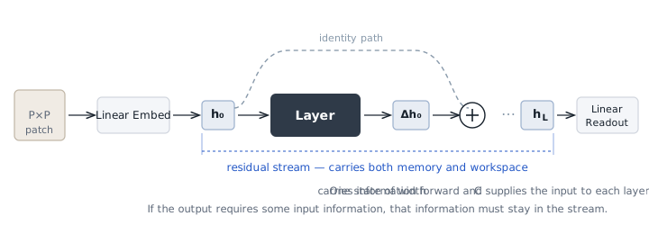
Now we revisit the advantage of -prediction from these two perspectives.
Noisy targets require a plain DiT's hidden states to retain noise-dependent input variation through the residual stream for the final readout, so that subsequent layers must compute on noisy representations. As patch size grows, more corruption-dependent pixel variation is packed behind each token, increasing the preservation pressure on its residual state. By contrast, a clean target concentrated in fewer directions reduces the demand on information-carrying capacity for the final readout.
More generally, the output target determines what information must be preserved through depth, and this preservation requirement shapes the representations learned along the residual stream. We call this requirement residual-stream burden.
Interactive The schematic summarizes this picture. Blue marks clean image structure, orange marks noise-dependent variation, and gray blocks are DiT blocks. The tabs compare a plain DiT under the two targets, decoupled designs that give the noise its own route, Hyper-Connections that widen the stream, and SiHC, which assigns each stream one subpatch. The particles sketch where information travels and are not measured activations. Use the tabs to switch designs, or open it full size.
Accordingly, the relevant low-dimensionality should appear in the patch space through which a DiT sees the image, and the relevant capacity should be the bandwidth of the persistent state that carries information across depth. Before examining both in Diffusion Transformers, we first visualize the burden with a toy experiment.
A toy example with residual FCNs
Following Li and He [5], the ground-truth data are a planar Swiss roll embedded in by an orthogonal matrix that is unknown to the model. We train toy flow-matching models to learn this distribution with a five-layer residual ReLU fully connected network (FCN) of width 256. The generation results are consistent with those reported by Li and He, as -prediction recovers the distribution and -prediction fails. Our focus, however, is on the internal states. Figure 2 shows that under -prediction the FCN concentrates residual-state variance in a few directions except at the highest noise level, whereas under -prediction it needs over a hundred directions to explain 90% of the variance by the last block. Even when the input is nearly clean, -prediction still spreads residual-state variance over many directions, so later layers receive broadly varying states.
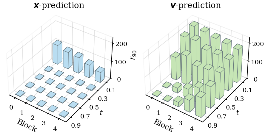
This toy experiment makes concrete how the prediction target shapes the internal representations in the residual stream. In the rest of this post, we examine this insight with Diffusion Transformers on real data.
The exploitable low-dimensionality is spectral concentration in patch space
We begin with the first question by identifying the exploitable low-dimensional structure in target patches, and then trace how this structure shapes input filtering and the resulting intermediate representations.
Spectral concentration in patch space
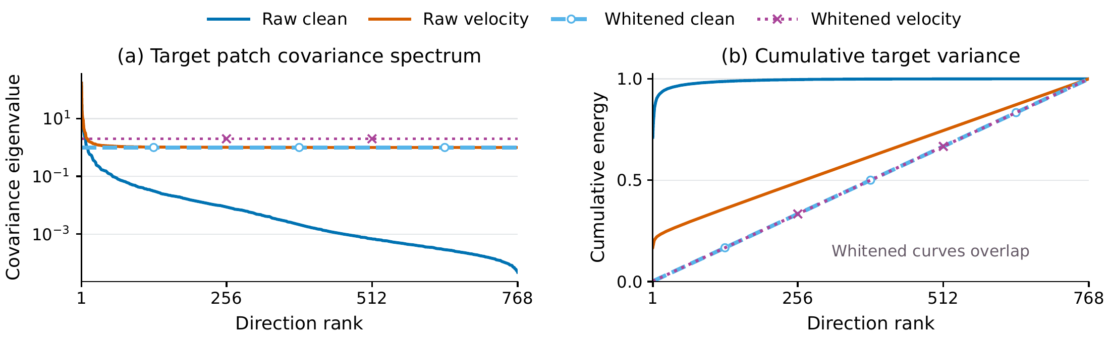
Low-dimensional patch structure is a longstanding theme in image modeling and denoising [9, 10]. A DiT processes noisy images patch by patch, so it is natural to ask how this geometry enters its training. For clean RGB patches in ImageNet , just 8 of 768 principal directions explain 90% of the variance () and already preserve recognizable image structure (Figure 3). We refer to this property as spectral concentration. The velocity target does not share it. Recall that flow matching [3, 4] interpolates between noise and data as , with for noise and for clean data, and that its target is the velocity . Because contains independent Gaussian noise, its variance spreads over almost all directions, and it requires 668 directions to reach the same fraction.
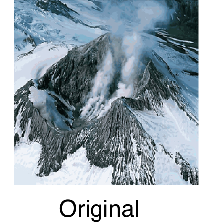
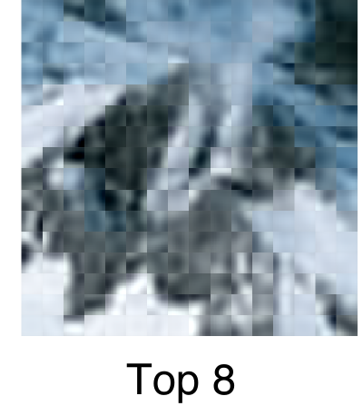
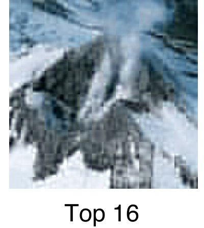
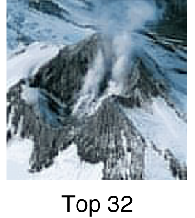
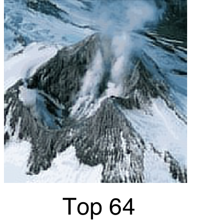
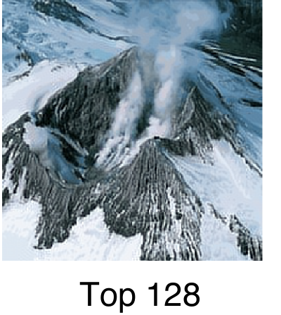
Clean patches are therefore low-dimensional in two senses. They lie near a low-dimensional manifold, as Li and He argue, and their variance concentrates in a few directions. To tell which of the two the network exploits, we whiten the clean patches with an invertible linear transform that sets every eigenvalue of the clean-patch covariance to one. Because the transform is invertible, it maps the clean-data manifold to another, smoothly equivalent manifold of the same dimension1. Whitening therefore removes the spectral concentration while preserving the manifold structure. We train the same DiT in the whitened space and map the generated samples back to pixel space for evaluation. If a low-dimensional manifold were sufficient, -prediction should succeed as before. Instead, its FID rises from 10.19 to 132.95, close to the 139.83 of pixel -prediction, and the whitened clean target needs 692 directions to explain 90% of its variance (Figure 4). This suggests that spectral concentration in patch space underlies the success of -prediction.
| Prediction target | Data space | FID ↓ | |
|---|---|---|---|
| Clean | Pixel | 10.19 | 8 |
| Velocity | Pixel | 139.83 | 668 |
| Clean | Whitened | 132.95 | 692 |
B-size plain DiTs, 200 epochs, ImageNet-, Heun-50. counts the target-patch directions needed to explain 90% of the variance.
How spectral concentration shapes representations
Following the toy experiment, we now show how patch spectral concentration is reflected in the representations along the residual stream.
Spectral concentration induces selective patch filtering. Since for , the optimal velocity estimator is
Under direct -prediction, the network must reproduce the noisy-input term, so its residual stream must carry corruption-dependent variation even along the many weak directions created by spectral concentration, where varies little. Under -prediction, the network outputs a clean estimate that is converted as . The noisy-input term is then supplied by this analytic long skip, so the backbone only needs , and the patch embedding, where the residual stream begins, can suppress these weak directions.
A best-affine calculation makes this difference concrete. For a clean patch with covariance eigenvalues , unit Gaussian noise and , the minimum-MSE affine predictions of the clean patch and of the velocity have variances
along the -th clean principal direction. As approaches zero, these approach 0 and 1, respectively. A weak clean direction thus contributes almost nothing to the clean estimate, yet it still contributes predictable variance to the velocity. On the ImageNet patch spectrum, the affine clean prediction consequently needs at most 7 directions to explain 90% of its variance at the evaluated noise levels, whereas the affine velocity prediction needs hundreds. In the whitened space every equals one, so the affine clean prediction has the same variance in every direction and is no longer concentrated.
| Clean coefficient | 0.1 | 0.3 | 0.5 | 0.7 | 0.75 | 0.9 |
|---|---|---|---|---|---|---|
| of affine clean prediction | 1 | 2 | 3 | 5 | 5 | 7 |
| of affine velocity prediction | 674 | 656 | 638 | 603 | 588 | 488 |
Computed from the ImageNet clean-patch spectrum.
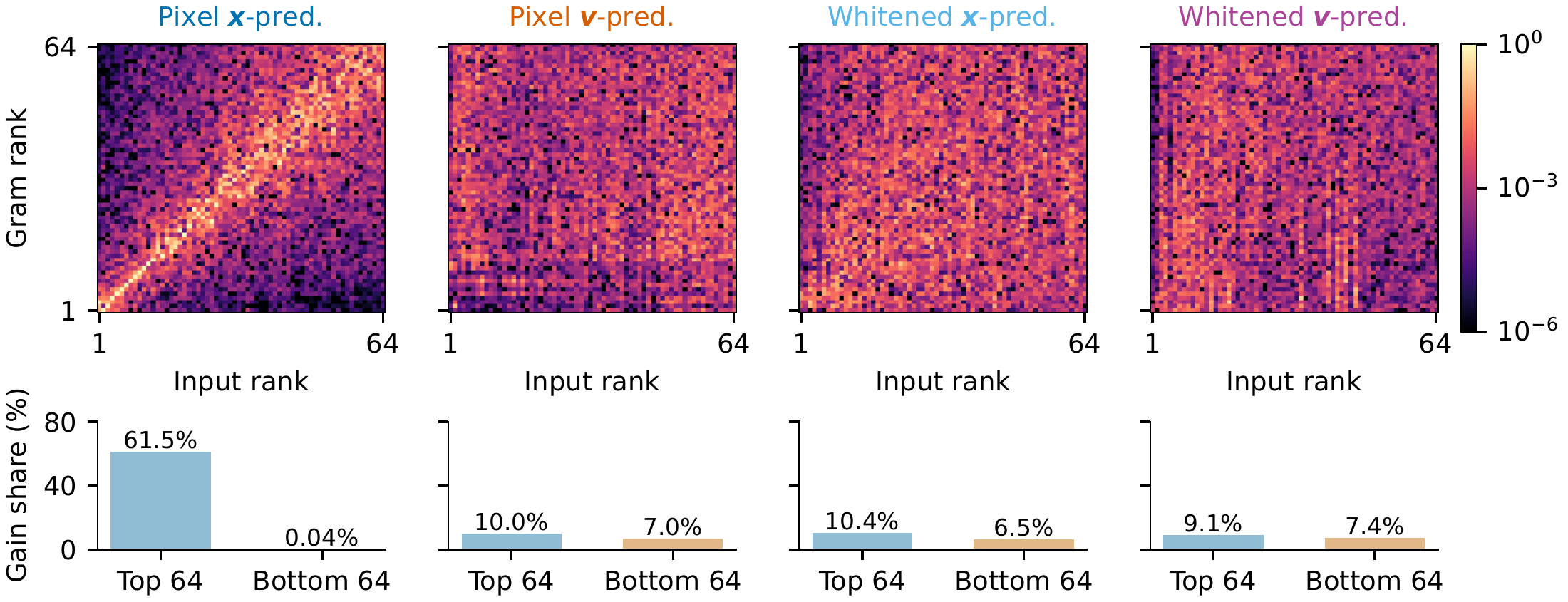
To examine this filtering in trained models, we measure the directional gain , which quantifies how strongly the patch embedding transmits variation along the clean-patch principal direction , and compare the eigenvectors of with these directions. Pixel -prediction assigns 61.5% of the total gain to the leading 64 clean-patch directions and only 0.04% to the trailing 64, compared with 10.0% and 7.0% for -prediction (Figure 5). Its embedding eigenvectors also align with the leading clean-patch directions. No such filtering emerges in the whitened space under either target.
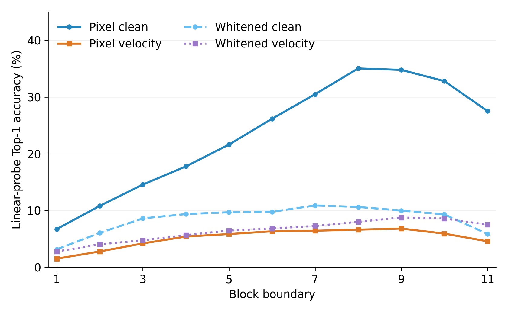
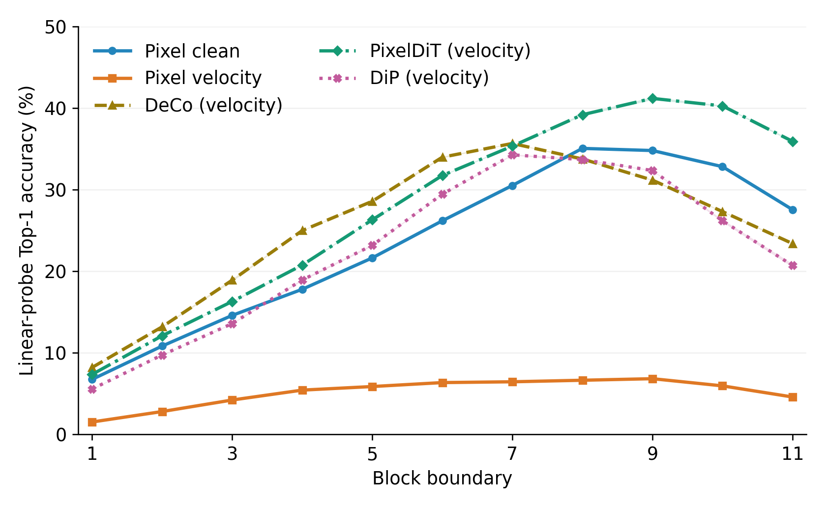
Noise burden and representation quality. For two noisy versions and of the same clean image, -prediction must keep their noise-dependent differences distinguishable in the residual stream, whereas -prediction does not, since the long skip supplies . This gives the backbone greater freedom to learn noise-robust representations. Earlier work shows that diffusion models learn features useful for recognition and correspondence [11, 12]. Our linear probes on frozen intermediate states show that pixel-space -prediction develops much stronger class features than -prediction, whereas both whitened models remain poorly class-readable, even under -prediction (Figure 6). Together with the embedding measurements, these results connect spectral concentration to selective noise filtering and stronger representations, whose quality is closely associated with generation quality [13].
Decoupled designs exploit low-dimensionality in the main stream
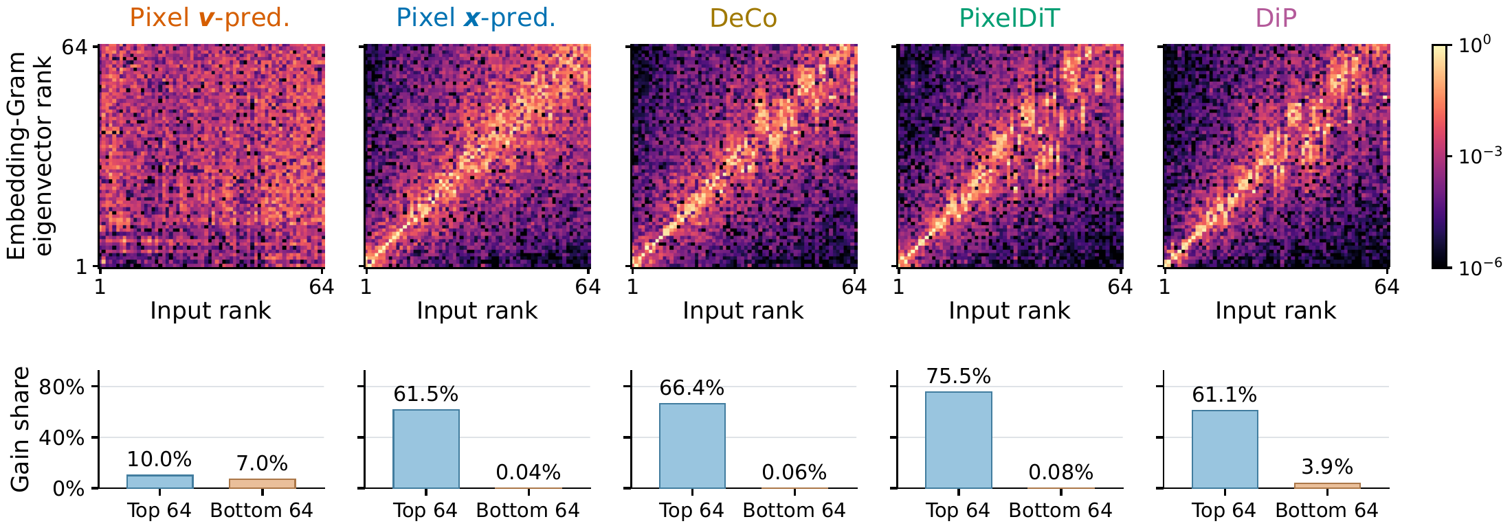
Decoupled architectures offer another way to exploit low-dimensional clean structure while predicting velocity. DeCo, PixelDiT and DiP [14, 15, 16] supply noisy pixels directly to a decoder conditioned on the main Transformer's features, allowing local noise-dependent variation to reach the output through a separate path. From this perspective, -prediction is a fixed, analytic form of decoupling, in which the long skip supplies the noisy input [5, 17]. We call the features passed to the decoder the semantic endpoint, which reflects the residual-stream burden on the main backbone of DiT blocks. All three B-size models train successfully under -prediction, reaching FID 6.33 to 13.31 compared with 139.83 for the plain DiT, and as expected, their semantic endpoints are far more concentrated than the velocity target (Figure 7). A low-dimensional interface thus emerges naturally through the end-to-end training of these decoupled designs.
Schematic In a decoupled design, a long skip takes the noisy pixels to the decoder, so the embedding of the main stream can filter out the noise.

As in a plain DiT with -prediction, this structure is reflected at the backbone's entrance and through its depth. The patch embeddings align with the leading clean-patch directions and suppress the trailing ones (Figure 8), while the intermediate states become much more class-readable than those of plain -prediction (Figure 9). At , their peak probe accuracies range from 34.26% to 41.18%, compared with 35.05% for pixel -prediction and 6.80% for pixel -prediction. These observations reconcile the decoder-based designs with -prediction, since both provide a separate path for the noisy input, accompanied by selective filtering and stronger representations in the main stream.
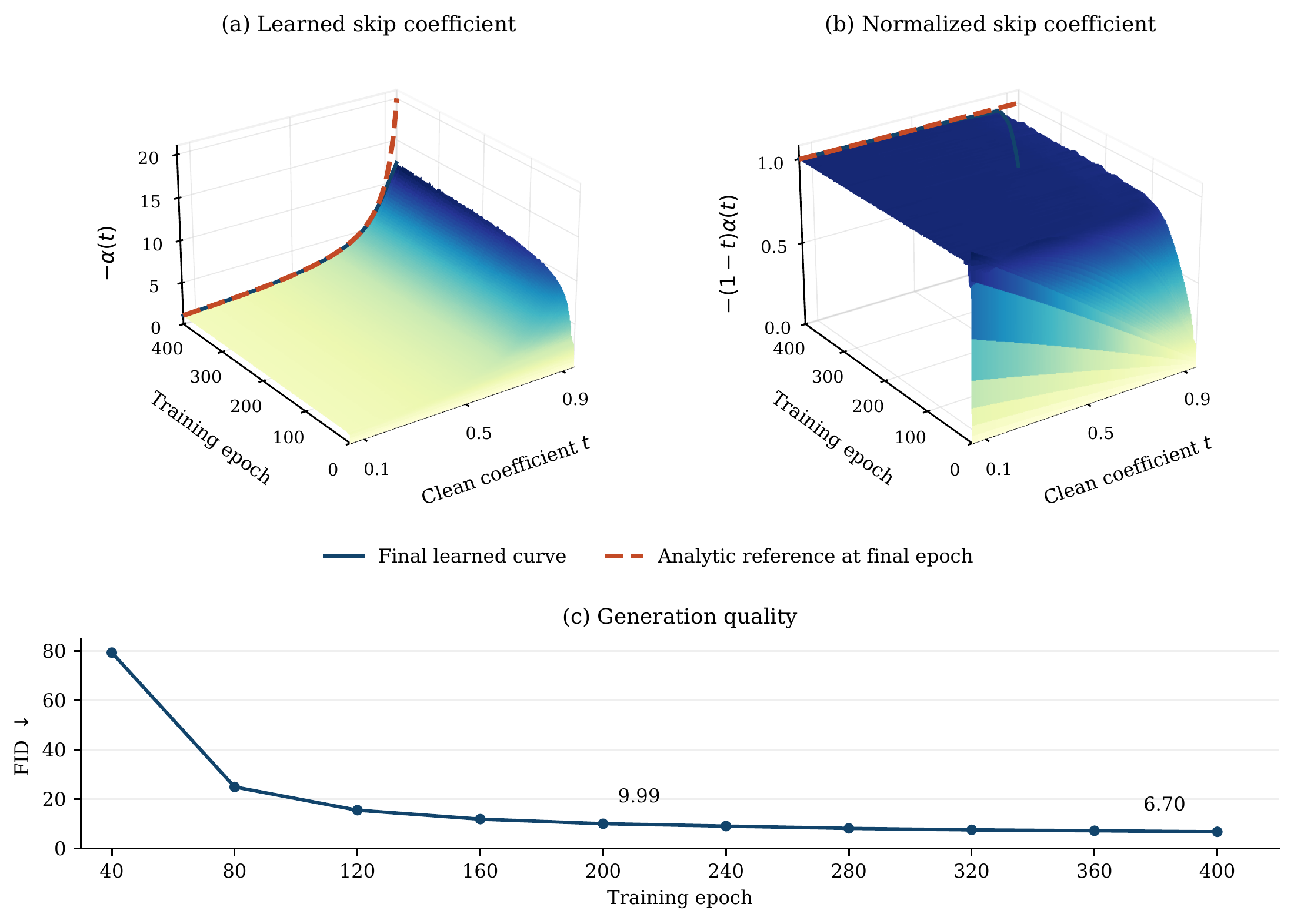
Even a zero-initialized scalar skip from the input to the output learns such a path. We augment the plain DiT as , initialize , and train with the velocity loss. The learned coefficient approaches , the input coefficient of the clean-to-velocity conversion , within two epochs at low and intermediate and across most noise levels by epoch 40. FID reaches 9.99 at 200 epochs, compared with 139.83 for the plain backbone (Figure 10). A related observation appears in -Diff, whose learned prediction parameter moves toward clean prediction in pixel space [18].
Together, these results connect patch geometry, prediction targets and architecture through residual-stream burden. The target-patch covariance spectrum serves as a measurable proxy for the size of this burden, since it describes how broadly target variation is distributed across directions. By this measure, the velocity target places a far larger burden than the clean target ( of 668 against 8). The architecture, in turn, determines how this burden is assigned to the main stream and to separate paths. With a separate pixel path, the semantic endpoints of decoupled models need only 35 to 309 directions at . When the burden instead stays on the main stream, as in plain -prediction, the stream itself may need more room. We next test whether expanding the residual stream helps accommodate this broader prediction demand.
The relevant capacity is residual-stream bandwidth
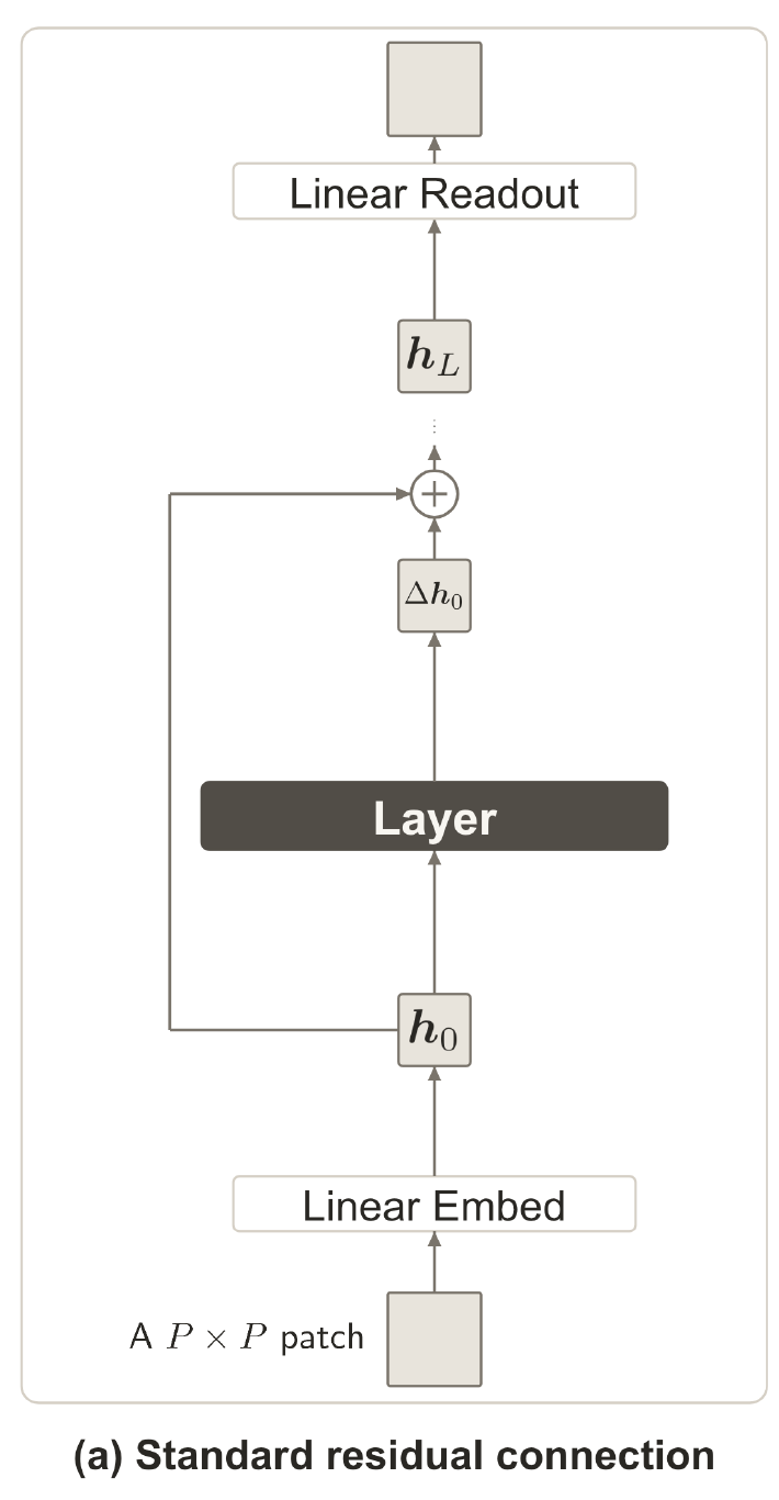
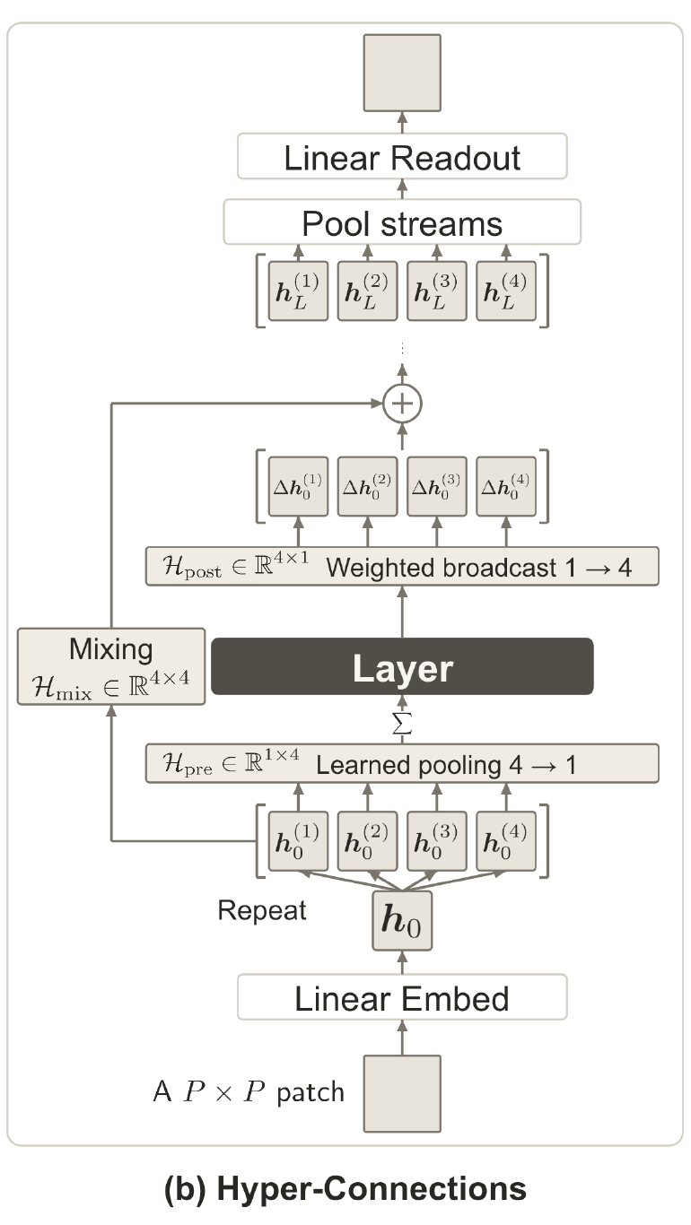
Having shown that separate pixel paths can relieve the main backbone of carrying noise to the final output, we now ask whether expanding the capacity of the persistent state lets the backbone accommodate this requirement internally. We call the width of the persistent state the residual-stream bandwidth. In a plain Transformer, increasing it also widens every attention and MLP computation, since the residual state itself serves as the workspace (Figure 11a). Hyper-Connections (HC) [19] separate the persistent state from the workspace, allowing us to expand the residual-stream bandwidth without widening those computations.
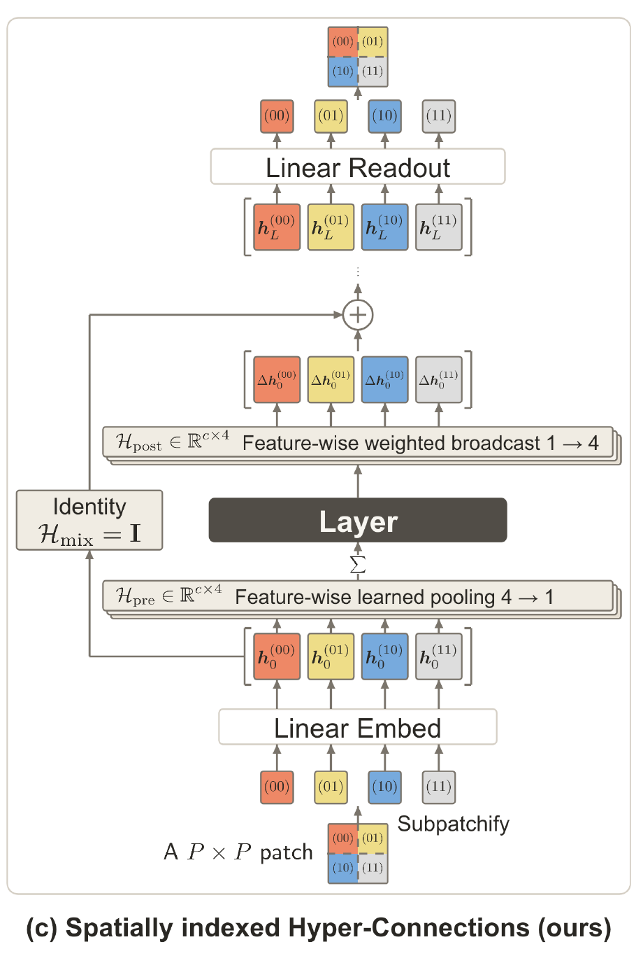
Expanding bandwidth with Hyper-Connections
HC replaces with persistent states , from which each update reads one width- workspace before writing its result back (Figure 11b),
The read map pools the states, the write map distributes the update, and the mixing map mixes the carried states. The residual-stream bandwidth thus becomes while the workspace width stays . We use mHC [20], a variant that keeps doubly stochastic for stable propagation through depth.
Schematic Hyper-Connections keep several persistent streams, each as wide as the plain one. Each DiT block reads from all of them and writes its update back, so the stream gains room without widening the computation.
The broader target spectrum of -prediction suggests a larger benefit from added bandwidth than for -prediction. We test this prediction with four-stream mHC, which expands the bandwidth at nearly unchanged parameters and GFLOPs while depth, token count and computational widths remain fixed. Besides pixel space, we run the test in the DINOv2-B [21] latent space used by RAE [22], whose 768-dimensional tokens match our pixel patches in size.
| Target | Plain FID ↓ | Four-stream mHC FID ↓ |
|---|---|---|
| Pixel, clean | 10.19 | 9.78 |
| Pixel, velocity | 139.83 | 25.36 |
| DINOv2-B, clean | 5.50 | 3.93 |
| DINOv2-B, velocity | 16.56 | 3.98 |
B-size models, 200 epochs, ImageNet-, Heun-50, CFG 2.9.
With this intervention, -prediction improves substantially. Its pixel-space FID falls from 139.83 to 25.36, whereas -prediction barely changes, and in DINOv2-B space the added bandwidth nearly closes the gap between the two targets. Residual-stream bandwidth is therefore a key resource for accommodating the burden of noisy prediction.
Spatially Indexed Hyper-Connections
Copied streams expand bandwidth but leave the division of the burden among streams to training. Spatially Indexed Hyper-Connections (SiHC) make this division explicit by assigning each persistent state the input and output of one subpatch, while attention and MLP layers read a shared workspace from all states, keeping the number of workspace tokens unchanged (Figure 11c). Three design choices realize this division.
- Local states carry local predictions. Each computational patch is divided into subpatches. Each state embeds only its noisy subpatch and predicts its local velocity, which reduces its prediction responsibility from to pixel coordinates, while the local predictions tile the full velocity patch.
- Identity carry keeps local detail available. With , each state retains its own carry path, independently of its contribution to the current workspace.
- Static feature-wise access connects local states to shared computation. Learned, input-independent read and write maps let each channel read its own combination of states and distribute its update with its own weights.
Read-back makes local information available to subsequent computation, and write-back distributes the resulting updates among the local prediction states.
Schematic In SiHC each stream embeds and predicts one subpatch, giving it a local prediction responsibility, while shared computation reads from all streams and writes updates back to them.
Each design choice improves velocity prediction. The table below tests these choices in sequence on a B-size backbone with computational patches and direct -prediction.
| Design | State region | Streams | FID ↓ |
|---|---|---|---|
| Plain DiT | 1 | 139.83 | |
| mHC, copied input | 4 | 25.36 | |
| mHC, local input and prediction | 4 | 13.25 | |
| + identity carry, static scalar maps | 4 | 11.50 | |
| + feature-wise maps (SiHC) | 4 | 10.10 | |
| + subpatches | 16 | 8.07 |
200 epochs. Parameters and GFLOPs remain nearly unchanged across the progression.
Assigning each of four streams its own input and prediction region lowers FID from 25.36 to 13.25 at the same bandwidth, demonstrating the value of smaller local responsibilities. Static scalar maps with identity carry improve FID further, and channel-specific read and write maps refine access to the local states without input-dependent connections. Dividing the patch into sixteen regions then expands the bandwidth while reducing each state's prediction responsibility to 48 pixel coordinates, bringing FID to 8.07, within the range of decoupled B-size models.
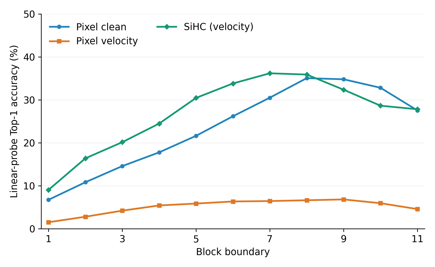
SiHC recovers clean-like class readability while predicting velocity. The SiHC workspace also develops much stronger class features than plain -prediction, tracking pixel-space -prediction through depth (Figure 12). At 50% input noise, its probe accuracy peaks at 36.18%, compared with 35.05% for pixel -prediction and 6.80% for pixel -prediction. Organizing the persistent state and its access thus recovers class-readable features without a separate pixel decoder.
The design scales to competitive generation quality. It also extends beyond the B-size analysis. With REPA [13], SiHC-XL reaches FID 1.71 on ImageNet , competitive with strong pixel-space models such as DiP (1.75), DeCo and PixelDiT (both 1.69), while retaining linear read and write maps in place of specialized decoders or cross-scale attention.
Late materialization makes the expanded state cheap to train. The static maps and the identity carry also make SiHC efficient to train. A literal implementation reads the full -stream state before every update and writes a new one after it, even though each attention or MLP update only uses a compact width- workspace. Because the maps are static and the carry is the identity, reads and writes compose across a stage. Every read can then be computed from the stage input and the compact updates accumulated so far, so the intermediate spatially indexed states are never materialized. They exist only logically, as the stage input plus the accumulated writes, and the wide state is written to memory once at the stage boundary. This late materialization allows exact kernel fusion and, compared with the unfused implementation of the same sixteen-stream B model, lowers peak training memory from 30.18 to 19.82 GiB and shortens the training step from 210.38 to 113.73 ms (H100 80GB, batch size 128, sublayerwise B model).
Interactive Eight updates of one SiHC stage. Colored stacks are the wide state and the gray bar is the compact workspace. In literal execution, every update reads the wide state from HBM and writes a new one back. In the fused stage, each workspace is computed from the stage input and accumulated compact updates, and the wide state is written once at the end. Literal autograd retains intermediate wide states for backward; fusion replaces these with the stage input and compact update history, reducing memory use. Click to pause. Open it full size.
Discussion
The high-level view of this work is to treat a neural network not merely as a function but as a system, in which a persistent state carries information across depth and computation reads from and writes to that state. As functions, the prediction targets are interchangeable, whereas in such a system each target also determines what the persistent state has to hold. When this includes information that later layers cannot build on, prediction and representation learning compete for the same state, and we call this competition friction. From this view, residual-stream burden explains a central difficulty in training diffusion models, because predicting a noisy target requires the residual stream to keep the noise and thereby induces friction with representation learning. Analyzing the patch space provides proxies for the size of this burden and shows why the issue becomes especially severe for high-dimensional data and large patches, where the noise spreads over far more directions. Through this lens, we reconcile recent progress in pixel-space diffusion, where changing the prediction parameterization and changing the architecture succeed for a common reason, namely relieving the main stream of the noise, and building on this understanding, we explore a complementary direction that accommodates the burden by expanding residual-stream bandwidth, with SiHC serving as an algorithmic probe.
Future directions
Viewing residual-stream burden through its friction with representation learning raises several questions.
Does gradient descent drift toward less friction? Selective filtering, concentrated semantic endpoints and the learned long skip all emerge without an explicit objective, which leads us to conjecture that whenever the architecture offers a path that carries the burden outside feature-building computation, gradient descent drifts toward solutions with less friction, consistent with a preference for simpler solutions. Testing this conjecture requires a way to characterize friction during training, for example as interference between the gradients that preserve the target and those that build features.
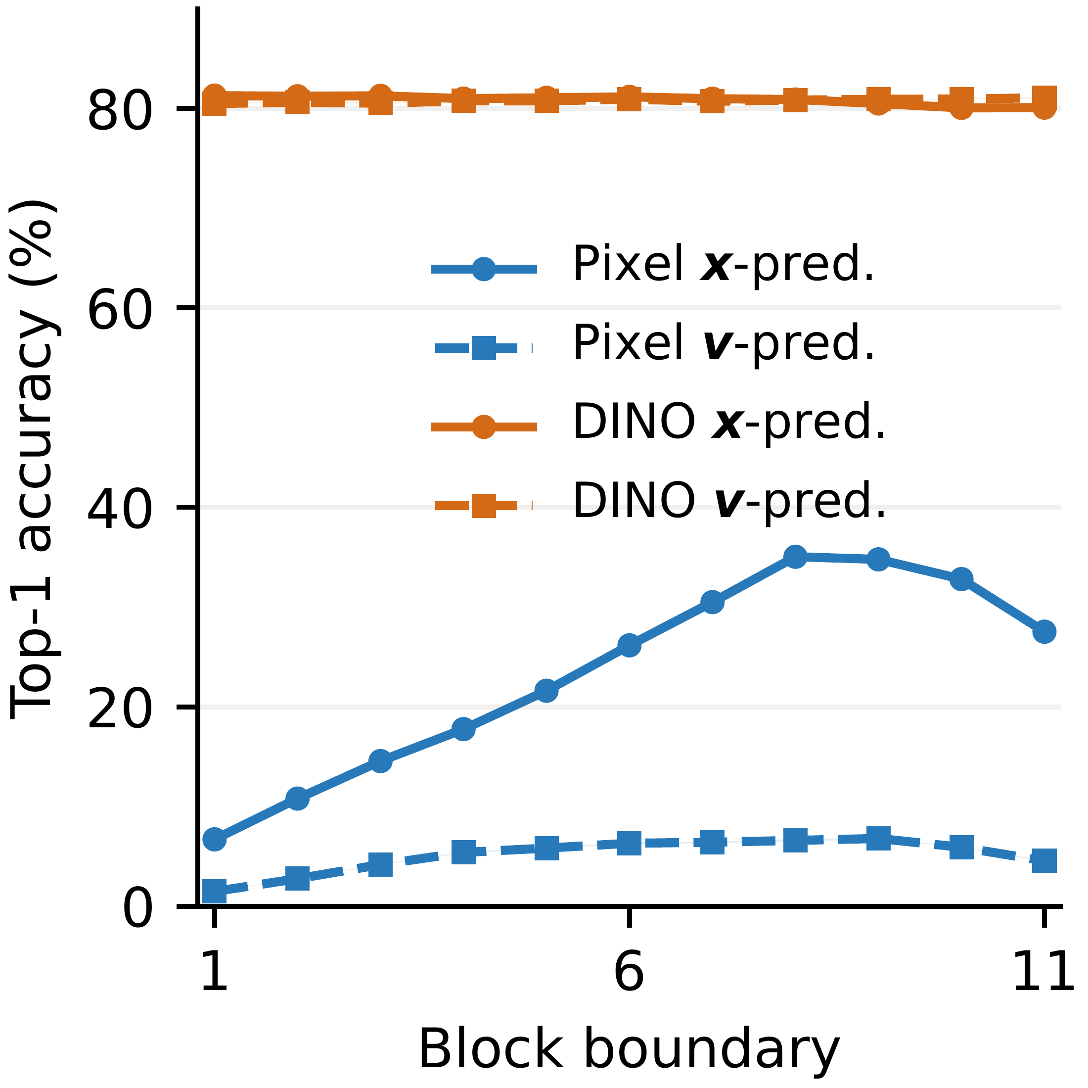
Can residual-stream burden benefit representation learning? When the target is itself a pretrained representation, as in RAE [22], the burden consists of features that later layers can build on, so carrying it may even facilitate representation learning. Our DINOv2-B experiments are consistent with this view, since the DINO and pixel velocity targets need a similar number of directions to explain 90% of their variance (651 and 668), yet both DINO models remain highly class-readable through depth while pixel -prediction does not (Figure 13). This contrast offers a possible reason for the fast convergence of RAE and invites studying diffusability, the question of which latent space suits diffusion models [23, 24, 25], from the perspective of neural network training.
When do generation and understanding reinforce each other? The same training perspective extends to unified models of generation and visual understanding, such as Janus [26], and recent unified models that generate within a shared semantic latent space, such as LatentUM [27], report improved alignment between the two tasks. Characterizing the burden that generation places on shared representations, and when this burden is compatible with understanding, may therefore help explain when the two tasks reinforce each other.
References
[1] Jonathan Ho, Ajay Jain, and Pieter Abbeel. Denoising Diffusion Probabilistic Models. NeurIPS, 2020.
[2] Tim Salimans and Jonathan Ho. Progressive Distillation for Fast Sampling of Diffusion Models. ICLR, 2022.
[3] Yaron Lipman, Ricky T. Q. Chen, Heli Ben-Hamu, Maximilian Nickel, and Matt Le. Flow Matching for Generative Modeling. ICLR, 2023.
[4] Xingchao Liu, Chengyue Gong, and Qiang Liu. Flow Straight and Fast: Learning to Generate and Transfer Data with Rectified Flow. ICLR, 2023.
[5] Tianhong Li and Kaiming He. Back to Basics: Let Denoising Generative Models Denoise. CVPR, 2026.
[6] William Peebles and Saining Xie. Scalable Diffusion Models with Transformers. ICCV, 2023.
[7] Ashish Vaswani et al. Attention Is All You Need. NeurIPS, 2017.
[8] Kaiming He, Xiangyu Zhang, Shaoqing Ren, and Jian Sun. Deep Residual Learning for Image Recognition. CVPR, 2016.
[9] Gabriel Peyré. Manifold Models for Signals and Images. Computer Vision and Image Understanding, 113(2):249–260, 2009.
[10] Kostadin Dabov, Alessandro Foi, Vladimir Katkovnik, and Karen Egiazarian. Image Denoising by Sparse 3-D Transform-Domain Collaborative Filtering. IEEE Transactions on Image Processing, 16(8):2080–2095, 2007.
[11] Weilai Xiang, Hongyu Yang, Di Huang, and Yunhong Wang. Denoising Diffusion Autoencoders are Unified Self-supervised Learners. ICCV, 2023.
[12] Luming Tang, Menglin Jia, Qianqian Wang, Cheng Perng Phoo, and Bharath Hariharan. Emergent Correspondence from Image Diffusion. NeurIPS, 2023.
[13] Sihyun Yu, Sangkyung Kwak, Huiwon Jang, Jongheon Jeong, Jonathan Huang, Jinwoo Shin, and Saining Xie. Representation Alignment for Generation: Training Diffusion Transformers Is Easier Than You Think. ICLR, 2025.
[14] Zehong Ma, Longhui Wei, Shuai Wang, Shiliang Zhang, and Qi Tian. DeCo: Frequency-Decoupled Pixel Diffusion for End-to-End Image Generation. CVPR, 2026.
[15] Yongsheng Yu, Wei Xiong, Weili Nie, Yichen Sheng, Shiqiu Liu, and Jiebo Luo. PixelDiT: Pixel Diffusion Transformers for Image Generation. CVPR, 2026.
[16] Zhennan Chen et al. DiP: Taming Diffusion Models in Pixel Space. CVPR, 2026.
[17] Hansheng Chen, Jan Ackermann, Minseo Kim, Gordon Wetzstein, and Leonidas Guibas. Asymmetric Flow Models. arXiv:2605.12964, 2026.
[18] Qing Jin and Chaoyang Wang. Revisiting Diffusion Model Predictions Through Dimensionality. arXiv:2601.21419, 2026.
[19] Defa Zhu et al. Hyper-Connections. ICLR, 2025.
[20] Zhenda Xie et al. mHC: Manifold-Constrained Hyper-Connections. ICML, 2026.
[21] Maxime Oquab et al. DINOv2: Learning Robust Visual Features without Supervision. Transactions on Machine Learning Research, 2024.
[22] Boyang Zheng, Nanye Ma, Shengbang Tong, and Saining Xie. Diffusion Transformers with Representation Autoencoders. ICLR, 2026.
[23] Ivan Skorokhodov, Sharath Girish, Benran Hu, Willi Menapace, Yanyu Li, Rameen Abdal, Sergey Tulyakov, and Aliaksandr Siarohin. Improving the Diffusability of Autoencoders. ICML, 2025.
[24] Jingfeng Yao, Bin Yang, and Xinggang Wang. Reconstruction vs. Generation: Taming Optimization Dilemma in Latent Diffusion Models. CVPR, 2025.
[25] Xingjian Leng, Jaskirat Singh, Yunzhong Hou, Zhenchang Xing, Saining Xie, and Liang Zheng. REPA-E: Unlocking VAE for End-to-End Tuning of Latent Diffusion Transformers. ICCV, 2025.
[26] Chengyue Wu et al. Janus: Decoupling Visual Encoding for Unified Multimodal Understanding and Generation. CVPR, 2025.
[27] Jiachun Jin, Zetong Zhou, Xiao Yang, Hao Zhang, Pengfei Liu, Jun Zhu, and Zhijie Deng. LatentUM: Unleashing the Potential of Interleaved Cross-Modal Reasoning via a Latent-Space Unified Model. arXiv:2604.02097, 2026.